Is Microsoft Excel too complicated? It doesn’t have to be. Excel uses formulas to pull in information to a single cell from others around it. These works like Excel shortcuts making life easier. If you know the right formulas, Excel doesn’t have to be complicated at all.
Here are 12 Excel formulas that are easy to remember and easy to apply. Some are basic formulas but others are advanced Excel functions that may sound tricky, so the best thing to do is to follow each example as it comes and then apply it to Excel as you read through the article.

1. The sum (SUM)
This allows you to add several figures, just like in school. There are two ways.
The first allows you to add cells in sequence (columns or rows). Just put =SUM(first cell:last cell) in the cell where you want to display the result.
Variant : This formula also allows you to add up all the numbers in a particular data set (multiple column numbers and multiple rows), taking the “first cell” as the top left, and the “last cell” as the bottom right.
The second method allows you to add (unrelated) cells individually. Just put =SUM(cell1;cell2;cell3;cell4) in the cell where you want to display the result.
Example :
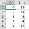
To add the contents of the column a eg. cell A1, enter =SUM (A1:A5) in the cell of your choice.
 To add the contents of the column a eg. cell A1, enter
To add all the numbers in the pivot table, enter =SUM (A1:B5) in the cell of your choice.
To add only the cells with a negative number like in cell b2, enter =SUM (A1;B2;B5) in the cell of your choice.
2. The “If Function” sum according to a specific criterion (SUM.IF)
A table can come in the form of a list of several items, which aren’t necessarily related. If the list is long, it can be difficult to find all the identical elements to add them one by one. To do this, you can ask Excel to find all these specific cases and make the sum using the formula =SUM.IF(range_cells;”test”;sum_range) . The “criterion” is the item type to be found in the table. The range_cells is the range of cells containing the relevant criterion. The sum_range is the range of cells where the numbers add up.
Example :
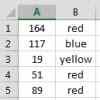
In this example, the criterion to look for is “red”. To calculate the total of the “reds” only, enter the following formula: =SUM.IF(B1:B5,red”,A1:A5) in the cell of your choice.
 In this example, the criterion to look for is “red”. To calculate the total of the “reds” only, enter the following formula:
Best apps and online tools to stay focused and be more productive
3. The sum according to several criteria (SUM.IFS)
A table can contain a lot of information. Excel can add data based on multiple criteria using a special formula: =SUMIFS(sum_range;range_criterion1;criterion1; range_criterion2;criterion2;….) . sum_range is the range of cells with the numbers to be added. range_criterion1 represents the range of cells containing the data with the first criterion, range_criterion2 being the second criterion, and so on. criterion1 is the first item type (criterion) to be found in the table, etc..
Example :
To find the number of points earned by the men on the yellow team, enter the following formula: SUMIFS (D1:D13,C1:C13,C1,B1:B13,B1) in the cell of your choice.
Variation : You don’t have to select the first and last cell from the column exactly, you can select an entire column . Instead of B1: B13, just enter B:B.
4. The sum of events based on a criterion (NB.IF)
Within a range of statistics, it’s sometimes interesting to know how many times a given event is repeated in a column. For this, we use the following function: =NB.SI(range_cell;”criterion”) . The range_cells is the range of cells containing the data. The criterion is the first criterion to be found in the table.
Example :
In the preceding table, you want to know how many women were involved in the game. Enter the following formula: =NB.SI (B1:B13, “Woman”) in the cell of your choice.
More about Windows 10
How to start Windows 10 in safe mode ►
How to turn on Bluetooth in Windows 10 ►
Windows 10 has a new free Microsoft Office app ►
Microsoft’s latest trick to get you to upgrade to Windows 10 ►
5. The sum of events based on several conditions (SUMPRODUCT)
This formula is used to extract a statistical answer to the question: how many times do these specific conditions occur in my table?
Answer: =SUMPRODUCT((range_criterion1=”criterion1″)*(range_criterion2=”criterion2″))
The range_criterion1 is the range of cells containing the data on the first criterion, the range_criterion2 corresponds to the second criterion, and so on. criterion1 is the first criterion to be found in the table, etc..
Example :
Taking the above table as an example, this formula allows us to say how many men were part of the yellow team. To do this, enter the following formula: =SUMPRODUCT((B1:B13=”Male”)*(C1:C13=”yellow”)) in the cell of your choice.
6. The sum of events between two specific values (SUMPRODUCT)
SUMPRODUCT is a statistical tool because it focuses on the number of times that certain conditions are met simultaneously. It allows you to find the number of times the figures are between two specific values, using the following formula: =SUMPRODUCT(range_cells>=minimum)*(range_cells<=maximum)) .
The range_cells is the range of cells containing the relevant figures. Minimum and Maximum are the two values between which our search results will appear.
Example :
In our previous table, we must find the number of players who scored between 150 and 200 points. To do this, enter the following formula: =SUMPRODUCT((D1:D13>=150)*D1:D13<=200)) in the cell of your choice.
7. Average (AVERAGE)
We probably don’t need to give you the definition of average. It’s very simple to achieve with the following formula: =AVERAGE(range_cells)
Example:
To calculate the average of all these numbers – in other words, the number that represents the typical value or mean of the figures, enter the following formula: =AVERAGE(A1:A6) in the cell of your choice. The range_cells is the range of cells containing the relevant figures.
8. Concatenate
The Concatenate formula is a simple string formula that will pull information from many different cells into one. A good example would be combining a person’s name, address, and date of birth into one column when previously the information had been spread across different cells.
To find. Concatenate you need to hit Formulas , then Text and Formulas , and then hit the Insert Function button. From there hit Category and Text . You’ll see it there as CONCAT.
5 Chrome extensions that can make you more productive
9. The maximum and the minimum (MAX and MIN)
Where you have a wide range of data, it can be quite a task to look for the largest or smallest number. Fortunately, Excel has a formula that looks for you. It’s very easy to apply since it appears as follows:
=MAX(range_cells)
=MIN(range_cells)
The range_cells is the range of cells containing the relevant figures.
Variation : you can also apply the search to multiple cell ranges.
The formulas then become:
=MAX(range_cells1;range_cells2)
=MIN(range_cells1;range_cells2)
Example :
In the preceding table, you’re looking for the greatest numerical value. Enter the following formula: =MAX(A1:A6) in the cell of your choice.
If you want the smallest numerical value, enter: =MIN A1:A6)
As you might guess, this formula is particularly useful if you’re working with very large tables.
10. Count up the number of cells with numbers (COUNT)
I don’t know why, but I always think of The Count from Sesame Street whenever I use this formula.
COUNT is a simple formula in Excel that simply counts up the number of cells in a given range that have numbers in them. Whereas the SUM function returns the total value of all the numbers in the range, COUNT is binary — it delivers a “1” if the cell has numerical contents and a “0” if it doesn’t.
This particular formula only works with numerical values. It’s cousin, COUNTA , does the same for all alphanumeric values in the cell and is ideal for testing whether cells in a range are “empty.”
Example Formula: =COUNT(A1:A20)
Five fantastic free alternatives to Microsoft Office
11. Get the Length of the Contents with LEN
Need to get a character count of the contents of a particular cell? Here comes LEN to the rescue! LEN counts up the total number of characters in a given cell. Note that this includes spaces!
Example Formula: =LEN(A1)
12. Recognize dates (DATEVALUE)
Excel can recognize certain serial numbers in select cells as being dates. For example, today’s date or the current date, whatever they may be, will be saved as an Excel serial number. You can use the =DATEVALUE(…) in an empty cell to change date figures to the Excel serial numbers and vice versa. This is useful for making date calculations, and sorting and filtering dates.
In short
While they may seem quite tricky at first, these Excel formulas will save you a lot of time if you use the software on a frequent basis, so it’s worth becoming familiar with them.
More about Excel
10 games for Microsoft Excel?! And free?! ►
What would Minecraft look like in Microsoft Excel? ►
7 tricks to use Microsoft Office free, without paying a cent ►
5 ways Microsoft Office is better than Google Drive ►
